From CT scanners to confusable characters: the prior art behind RaySpace

RaySpace measures glyph similarity by casting rays through font vector outlines at multiple angles and comparing the intersection patterns. It found 250,000+ confusable character pairs across 245 fonts. This post covers the two questions that naturally follow: where did the technique come from, and has anyone done something similar?

The answers turn out to be “a surprisingly deep well of prior work across unrelated fields” and “not really, but the pieces existed.”

Part 1: Where the idea came from

The ray as a geometric probe

The foundational insight is older than computer graphics itself.

Arthur Appel at IBM published “Some Techniques for Shading Machine Renderings of Solids” in 1968. He proposed casting a ray from a camera through each pixel into a 3D scene to determine what surface that pixel sees. For each hit, a secondary ray was cast toward the light source to determine shadow. Appel inverted the physics: instead of tracing photons from the light (most of which never reach the camera), he traced rays backward from the camera and asked “what does this pixel see?”

The insight that matters here is not the rendering application. It is the abstraction. A ray is a geometric query: an origin, a direction, and the question “what does this hit, and how far away?” That abstraction generalises to any domain where you want to probe geometry along a straight line. Sonar, radar, CT scanning, acoustic modelling, and font outline analysis are all variations of Appel’s probe.

Turner Whitted at Bell Labs extended Appel’s work in 1980 with “An Improved Illumination Model for Shaded Display”. At each surface intersection, Whitted’s algorithm spawns secondary rays (reflection, refraction, and shadow rays), creating a recursive tree. The key insight for RaySpace is that a ray’s full interaction history, not just its first hit, carries rich information. When a ray passes through a glyph outline, the sequence of all intersections along the ray (enter stroke, exit stroke, enter next stroke, exit next stroke) encodes the glyph’s cross-sectional topology at that angle.

Carmack’s constraint trick

John Carmack at id Software made raycasting fast enough for real-time consumer hardware in 1992.

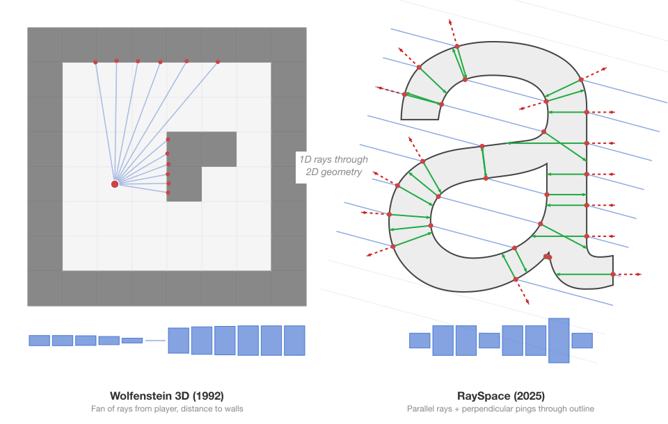
Wolfenstein 3D defined its world as a 2D grid map. For each vertical column of pixels on screen (320 columns at 320x200 resolution), the engine cast a single ray from the player’s position into the 2D map using a DDA (Digital Differential Analyzer) for efficient grid traversal. When the ray hit a wall cell, the distance determined the wall height drawn in that column. Nearby walls appeared tall, distant walls appeared short. The illusion of 3D from a fundamentally 2D data structure.

The constraints that made this work on a 386 at 16-33 MHz with no floating point unit and no GPU:

All walls on a grid, perpendicular to the floor, same height
No vertical look (camera locked to horizon)
One ray per screen column, not per pixel
Integer and fixed-point arithmetic throughout
DDA traversal stepping from grid line to grid line, never missing a wall

Doom (1993) moved beyond grids to arbitrary 2D polygonal layouts with BSP (Binary Space Partition) trees, but the conceptual DNA is the same: derive a spatial understanding of geometry from 1D ray queries against a 2D structure.

The paradigm maps directly onto RaySpace. Carmack’s 2D floor plan is the glyph outline. His parallel rays are the 50 rays per angle. His wall-hit distances are intersection positions. His screen columns are the per-ray signature entries. The core trade is identical: accept geometric constraints (outlines are 2D, rays are 1D) and gain enough structural information to characterise the shape without ever reconstructing a full image.

Wolfenstein 3D casts a fan of rays from a player into a 2D grid map and measures distance to walls. RaySpace casts parallel rays through a glyph outline and records intersection patterns, with perpendicular ping rays measuring stroke width at each crossing. Both derive structural understanding from 1D rays through 2D geometry.

Ambient occlusion: the ancestor of ping rays

Ping rays (the perpendicular probes that measure stroke width at each intersection) have a direct ancestor in computer graphics.

The concept of measuring how exposed or enclosed a surface point is by casting rays outward was explored by Zhukov, Iones, and Kronin in their 1998 paper “An Ambient Light Illumination Model”. For each point on a surface, imagine the hemisphere of directions along the surface normal. Cast rays into that hemisphere. The fraction that hit nearby geometry is the occlusion value. A point deep inside a crevice is heavily occluded. A point on a flat, exposed surface is not.

Hayden Landis at Industrial Light and Magic brought ambient occlusion to film production, presenting the technique at SIGGRAPH 2002. ILM used it on Pearl Harbor (2001) and Star Wars: Episode II (2002). The mathematical formulation is a cosine-weighted integral over the hemisphere:

A O (p) = \frac{1}{π} \int_{Ω} V (p, ω) \cdot (n \cdot ω) d ω

where $V$ is a visibility function (0 if the ray hits geometry, 1 if it escapes). In practice, this is approximated by Monte Carlo sampling: fire 16-256 random rays, count how many are blocked.

Vladimir Kajalin at Crytek took this further in 2007 with Screen-Space Ambient Occlusion (SSAO), debuting in CryEngine 2 and the game Crysis. The key insight: you do not need the actual 3D scene geometry to approximate AO. The depth buffer, which the GPU already computes during normal rendering, contains enough geometric information. SSAO samples nearby pixels in the depth buffer, checks which ones are “in front of” the current point, and estimates occlusion from that. This made AO feasible in real time for the first time. Martin Mittring presented the technique at SIGGRAPH 2007 and wrote it up in more detail in ShaderX7 (2009).

SSAO demonstrates something relevant to RaySpace: you can extract meaningful geometric information from a reduced-dimensionality representation of geometry rather than from the full model. RaySpace similarly works not with the full complexity of font outlines in their original cubic Bezier form but with a discretised probe: rays at regular intervals, producing distance values.

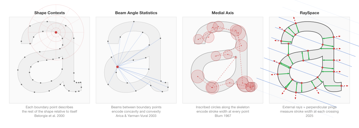
The connection to ping rays is direct. Ambient occlusion asks “how enclosed is this surface point?” by firing rays outward and measuring what fraction hit nearby geometry. A ping ray asks “how wide is this stroke?” by firing a single ray perpendicular to the glyph outline, into the interior, and measuring how far it travels before hitting the opposite wall. AO integrates over a hemisphere to produce a scalar darkness value. Ping rays sample along a contour to produce a vector of distances. The principle is identical: cast a ray from a surface, measure how far it goes before hitting something, and use the distance as a geometric descriptor.

Acoustic ray tracing: rays as fingerprints

Sound engineers discovered the fingerprint analogy decades before RaySpace applied it to glyphs.

Allred and Newhouse proposed using Monte Carlo ray tracing for architectural acoustics as early as 1958 in the Journal of the Acoustical Society of America. Krokstad, Strom, and Sorsdal at the Norwegian Institute of Technology published the first computational implementation in 1968: “Calculating the Acoustical Room Response by the Use of a Ray Tracing Technique” in the Journal of Sound and Vibration. They fired rays from a sound source, reflected them off walls according to the law of reflection, and collected arrival times and energies at a receiver point.

The result is an impulse response: a compact time-domain signal that characterises the room’s geometry. Fire a short burst of sound and record what comes back. The direct sound arrives first. Then first-order reflections from nearby walls. Then second-order, third-order, blending into a reverberant tail. The pattern encodes everything: room size, shape, surface materials, volume. Two rooms with identical impulse responses are acoustically indistinguishable. You can predict how any sound will behave in a room by convolving the dry signal with the impulse response.

Wallace Clement Sabine at Harvard laid the quantitative groundwork in 1898, deriving the Sabine equation for reverberation time ( $R T_{60} = 0.161 \cdot V / A$ ). He was consulted on the design of Boston Symphony Hall (1900), one of the first concert halls designed with scientific acoustic principles. Manfred Schroeder at Bell Labs (1965) introduced the integrated impulse response method and maximum-length sequence (MLS) measurement technique, replacing starter pistols with repeatable pseudorandom noise.

Allen and Berkley (1979) developed the image source method as a complementary approach: for each reflecting surface, create a mirror image of the sound source, and compute specular reflection paths deterministically. Modern acoustic software (ODEON, CATT-Acoustic, Steam Audio, Microsoft Project Acoustics) uses hybrid approaches: image sources for early reflections where precision matters, stochastic ray tracing for late reverberation where statistical accuracy suffices.

The analogy to RaySpace is direct, and familiar territory for anyone who has studied acoustics or music production. Krokstad fires rays into an enclosed 3D space and uses the pattern of reflections to characterise the room’s geometry. RaySpace fires rays through an enclosed 2D space (a glyph interior) and uses the pattern of intersections to characterise the glyph’s geometry. A small hard-walled room produces short, dense reflections; a cathedral produces long, sparse ones. A narrow stroke produces short ping distances; a wide bowl produces long ones. The acoustic impulse response is to a room what the RaySpace distance vector is to a glyph: a compact, comparable representation of spatial geometry derived from ray interaction data.

Sonar: the literal namesake

The “ping ray” in RaySpace is named after sonar.

Active sonar was developed by multiple groups during and after World War I. Paul Langevin and Constantin Chilowsky in France built the first practical underwater detection system using piezoelectric quartz transducers (1915-1918). Reginald Fessenden in the US built the first working echo-ranging system in 1914, the Fessenden oscillator, which could detect icebergs at two miles. Robert Watson-Watt in the UK developed the analogous electromagnetic version (radar) in 1935 for the Chain Home system.

The principle is the same across all of these: emit a pulse of directed energy, wait for it to return, and infer geometry from the delay and characteristics of the return signal. A sonar ping measures “how far is the nearest obstacle in this direction?” A RaySpace ping ray measures “how far is the opposite wall of this stroke?” Both are distance-measuring probes fired from a surface into an unknown geometry.

Medical ultrasound applies the same principle at shorter range and higher frequency. Ian Donald published the landmark clinical paper in The Lancet in 1958. The technology descends directly from sonar: a transducer emits a short ultrasonic pulse into tissue, and at each boundary between tissue types (different acoustic impedances), part of the pulse reflects back. The time delay of each echo gives the depth of each boundary. Scanning the beam builds a 2D cross-sectional image. The physics is identical to sonar; the domain is different.

Computed tomography: the mathematical guarantee

The deepest connection is to CT scanning, because it provides the theoretical proof that multi-angle ray probing works.

Godfrey Hounsfield at EMI Laboratories built the first clinical CT scanner in 1971. The first brain scan was performed on 1 October 1971 at Atkinson Morley Hospital in London. Allan Cormack at Tufts University had independently developed the mathematical reconstruction theory in 1963-1964, unaware of earlier work by Radon. Hounsfield and Cormack shared the 1979 Nobel Prize in Physiology or Medicine.

The CT principle: fire X-rays through the body at many angles. At each angle, multiple parallel rays sample across the body. A detector on the opposite side measures how much each ray was attenuated (the line integral of tissue density along the ray’s path). From the complete set of line integrals at all angles, a reconstruction algorithm (filtered back-projection) computes the 2D cross-sectional density map.

The raw CT data, organised as angle vs. detector position, is called a sinogram (because a point in the original image traces a sinusoidal curve in the angle-offset space). This is formally analogous to a RaySpace descriptor organised as angle vs. ray position vs. intersection pattern.

The formal correspondence:

CT scanning	RaySpace
X-rays fired through the body	Rays fired through a glyph outline
Multiple angles (hundreds)	36 angles (every 5 degrees)
Attenuation line integral per ray	Intersection count + positions per ray
Sinogram (angle x offset)	Ray descriptor (angle x ray index)
Reconstruct internal structure	Characterise glyph structure
Compare scans to detect pathology	Compare descriptors to detect confusability

Johann Radon proved the mathematical foundation in 1917: “On the determination of functions from their integral values along certain manifolds”, published in the Berichte of the Saxon Academy of Sciences. Radon showed that a 2D function can be uniquely reconstructed from the complete set of its line integrals. This was pure mathematics; Radon had no applied application in mind. The paper was largely forgotten until CT scanning made it suddenly, profoundly relevant in the 1970s.

Radon’s uniqueness theorem is why multi-angle ray probing works for shape comparison. If two sets of line integrals (projections) are similar, the underlying shapes must be similar. Even a coarse discrete approximation (36 angles, 50 rays per angle = 1,800 total) captures enough of the Radon transform to distinguish most shapes. RaySpace does not reconstruct the glyph from its projections; it compares the projections directly. This is valid because Radon’s theorem guarantees the projections contain all the information.

The letter "a" probed at four angles (0, 30, 60, 90 degrees). Each angle produces a different intersection pattern, shown as crossing counts in the strip below. Horizontal rays pass through the bowl and stem uniformly; diagonal and vertical rays reveal the internal structure of the counter and the stem-bowl junction. This is a discrete sinogram.

The accidental convergence

None of this was planned from the start. The raycasting filter existed as a crude pre-filter (count intersections, reject pairs with different topology, pass survivors to SDF). The decision to add more layers of information per ray (positions, crossing angles, ping distances) was driven by specific failures (the dot problem, the open-vs-closed problem). Only after ping rays were working did the connections become visible. A perpendicular probe from the outline surface measuring stroke width is ambient occlusion. The multi-angle intersection pattern is a Radon sinogram. The aggregate distance vector is an impulse response.

The technique is new in its application. Nobody has raycasted font outlines for confusable detection before. But the principles are between 50 and 100 years old.

Part 2: The confusable detection landscape

A field stuck on pixels

Every published homoglyph detection system works on rendered images. The approach is always the same: render characters to bitmaps, apply some form of image comparison (pixel differencing, SSIM, CNN embeddings, perceptual hashing), produce a similarity output. The variation is in the model, not the representation.

Here is what exists, chronologically.

Roshanbin and Miller (WISE 2011) published “Finding Homoglyphs,” one of the earliest demonstrations that visual similarity detection could find homoglyphs beyond the Unicode confusables list. Pixel-based bitmap comparison, single font (GNU Unifont), binary outcome. No continuous scores, no per-font analysis.

Woodbridge, Anderson, et al. (IEEE SPW 2018) built “Detecting Homoglyph Attacks with a Siamese Neural Network.” Renders domain names as images, feeds them to a Siamese CNN, outputs embedding vectors. Euclidean distance between embeddings gives similarity. 13-45% ROC AUC improvement over string-distance baselines. The innovation was applying neural networks; the limitation was operating at the domain level (full domain string images), not character-level pairwise comparison.

Suzuki et al.’s ShamFinder (IMC 2019) is the closest to RaySpace in ambition, if not in method. Its SimChar module renders every Unicode character as a 32x32 bitmap in GNU Unifont, computes the sum of absolute pixel differences between every character pair, and declares pairs with a difference of 4 pixels or fewer as homoglyphs. It found 13,208 pairs from 52,457 characters, over 20 times more than confusables.txt at the time. ShamFinder then used these pairs to detect phishing domains in the wild. The limitations are fundamental: one bitmap font at low resolution, a binary threshold with no continuous scoring, no per-font analysis (a pair that is confusable in Arial but not in Courier New gets the same treatment), and no multi-character support.

Deep Confusables (Munoz and Hernandez, HITB 2019) used VGG16 transfer learning on rendered character images to build a confusable dictionary. Released as the deep-confusables Python package. Generated fake domains that bypassed Chrome and Firefox IDN policies. Single font, binary classification.

Deng, Linsky, and Wright (IEEE ISI 2020) trained a CNN with triplet loss to produce character embedding vectors. Cosine distance between embeddings gives a continuous similarity score. They predicted 8,452 previously unrecorded homoglyphs with 0.97 average precision and attempted clustering homoglyphs into equivalence classes (0.592 mBIOU). This is the most sophisticated single-font pixel approach in the literature; the embedding-based continuous similarity is more nuanced than SimChar’s binary threshold. But it is still one font, one rendering, no per-font differentiation, no multi-character confusables.

Majumder et al. (MDPI 2020) built an ensemble of shallow CNNs for homoglyph recognition. 99.72% accuracy, 100% recall on one variant. Classification task, not scoring: binary “is this a homoglyph pair?” with no continuous output.

GlyphNet (Gupta et al., 2023) used an attention-based CNN on 256x256 domain-name images. A dataset of 4 million domain images. Its most useful finding was negative: ImageNet transfer learning (VGG16, ResNet18/34/50) scored only 63-67% accuracy on glyphs. Standard feature extractors trained on natural images (dogs, cars, landscapes) do not transfer to the high-contrast, geometric world of typographic shapes. Greyscale outperformed colour; stripping colour information preserves edge detail better through resizing. These findings validated simpler, non-neural approaches.

PhishHunter (Computers and Security, 2023) used a Siamese neural network on domain-name images with WGAN-GP for class imbalance. Domain-level detection, pixel-based. VizCheck (IEEE, 2024) took an OCR-based approach: render domains, run OCR, compare the “perceived” text with the actual text. Creative use of OCR as a visual similarity proxy, but still fundamentally pixel-based and domain-level.

At the industry end, Infoblox (2020) deployed a CNN classifier at DNS scale using Amazon SageMaker. Two stages: an offline CNN builds a Unicode-to-ASCII character map by comparing rendered images, then an online stream matches DNS queries against target domains using the map. 96.9% accuracy after hyperparameter tuning. Over 60 million resolutions of homograph domains detected. It is the most industrially deployed homoglyph detection system found, and entirely pixel-based. Netcraft documented active rn/m phishing campaigns in 2024 but detects them with string pattern matching.

How the browsers actually do it

Chrome and Firefox perform no geometric computation. Zero visual analysis.

Both use ICU’s USpoofChecker API, which implements the skeleton algorithm from UTS #39. The skeleton normalises a string by: NFD normalisation, removing ignorable characters, replacing each character with its confusable mapping from confusables.txt, normalising again. Two strings are confusable if their skeletons match. Chrome adds a 13-step algorithm on top: script mixing rules, skeleton matching against a global top domains list, and Cyrillic/Greek/Latin restrictions. But the confusable detection itself is pure lookup table.

Firefox explicitly delegates whole-script confusable handling to domain registries. Its position: “up to registries to make sure customers cannot rip each other off.”

The Unicode Consortium maintains an ML confusables generator for Han characters: triplet-loss CNN embeddings on rendered images. This is the pipeline that feeds confusables.txt. The original confusables.txt curation process was partly automated (a program compared characters sharing identical glyphs within a font) and partly manual volunteer review from contributors at Google, IBM, and Microsoft. The specific methodology for the automated font comparison was never documented publicly.

The rn/m substitution is the textbook multi-character confusable. It appears in every homoglyph paper as a motivating example. Marcet and Perea (2018) published psycholinguistic experiments in the Journal of Experimental Psychology demonstrating that “rn” is processed as “m” during reading: “docurnent” primed “DOCUMENTO” nearly as effectively as “documento” itself, with only 10-19ms response time difference. The finding that multi-character confusables fool the human visual system is empirically established.

But nobody has automated the search. Every source either cites rn/m as a known anecdote, detects it with a hand-coded string substitution rule, or validates it with a perceptual study. dnstwist, the most widely used domain permutation tool, generates homoglyph substitutions from a curated lookup table and treats each character independently. No multi-character composites.

No published system has done what RaySpace’s bigram pipeline does: systematically enumerate all two-character Latin sequences, concatenate their font outlines, compare against all single-character targets in 245 fonts, and discover which bigrams are geometrically confusable at per-font resolution. The 571,753 multi-character pairs, including cross-script discoveries like Latin “oy” matching Cyrillic uk (U+0479) at distance 0.000 in Helvetica, are entirely without precedent in the literature.

What does not exist

Synthesising everything above into a gap analysis:

Capability	State of the art	RaySpace
Input representation	Rendered pixels (32x32 to 256x256)	Exact vector outlines (Bezier curves)
Similarity output	Binary (most) or single-font embedding distance	Continuous per-font distance scores
Font awareness	Single font (GNU Unifont, or one system font)	245 fonts with per-font results
Multi-character	Anecdotal (rn/m cited, never searched)	571,753 discovered pairs
Scale	13,208 pairs (ShamFinder, 2019)	250,000+ single-char, 571,753 multi-char
Interior geometry	Not captured (pixels only)	Stroke width, counter depth (ping rays)

Part 3: The shape descriptor family tree

Confusable detection may be stuck on pixels, but the shape analysis community has spent decades building descriptors that characterise 2D forms. Several are conceptually related to what RaySpace does, some strikingly so. Understanding these relationships positions RaySpace in its mathematical context and explains why certain design choices work.

Four shape descriptors applied to the same glyph. Shape contexts (2000) describe each boundary point relative to all others. Beam angle statistics (2003) measure angles between lines connecting boundary points. The medial axis (1967) fits inscribed circles along the stroke skeleton. RaySpace (2025) casts external parallel rays and fires perpendicular pings at each crossing to measure stroke width.

The Radon transform: RaySpace’s mathematical foundation

The most important connection in this entire survey.

Johann Radon was an Austrian mathematician (born 1887, Decin, Bohemia; died 1956, Vienna). In 1917 he published “On the determination of functions from their integral values along certain manifolds” in the proceedings of the Saxon Academy of Sciences. He proved that a 2D function $f (x, y)$ can be uniquely reconstructed from the complete set of its line integrals:

R [f] (t, θ) = \int_{L (t, θ)} f (x, y) d s

where $L (t, θ)$ is the line at perpendicular distance $t$ from the origin, at angle $θ$ . The output $R [f]$ is a 2D function of angle and offset called a sinogram (a point in the original image traces a sinusoidal curve in sinogram space).

Radon’s inversion theorem says: if you know $R [f]$ for all $t$ and $θ$ , you can recover $f$ exactly. The inversion involves back-projection (smearing each projection back across the image) combined with a filtering step. This is the filtered back-projection algorithm used in every clinical CT scanner.

The connection to RaySpace is precise. Consider a glyph as a binary function $f (x, y) = 1$ inside the filled outline, 0 outside. The Radon transform of this function along a line gives the total chord length through the filled interior. RaySpace fires the same lines (at 36 angles, 50 offsets per angle) but instead of computing the chord length integral, it records the boundary crossings, where the line transitions from outside to inside and back. The intersection count is a topological version of the Radon integral: it tells you how many separate regions the line passes through, not their total width.

This distinction matters. A ray through a single thick stroke and a ray through two thin strokes of the same total width produce the same Radon integral but different RaySpace counts (2 vs. 4 intersections). RaySpace preserves topological information that the continuous Radon transform discards by integrating.

Shape descriptors built on Radon:

Tabbone, Wendling, and Salmon (Computer Vision and Image Understanding, 2006) developed the R-transform: collapse the sinogram to a 1D function by computing the squared L2 norm of each column (total squared Radon energy per angle). Translation-invariant by construction. Rotation shifts the function cyclically. Applied to technical symbol and graphical shape recognition.

The DTW-Radon descriptor (IJPRAI, 2013) preserves more spatial information by applying dynamic time warping to the full sinogram columns rather than collapsing to norms. Good results on graphical symbols, handwritten characters, and footwear prints. Robust to deformation and degradation.

The Histogram of Radon Transform (HRT) computes per-angle histograms of Radon values, providing finer resolution than the R-transform while maintaining invariance properties.

The Radon transform has been applied directly to character recognition: Arabic characters, postal characters with PCA, and DTW-Radon for character classification. But all of these operate on rasterised images and aim for character recognition (what letter is this?), not pairwise similarity scoring between different characters.

RaySpace extends the Radon framework in three ways no prior method combines:

Vector outlines, not raster images. The line integrals are computed analytically against Bezier curves via polynomial root-finding, not numerically against pixel grids. No discretisation error, no resolution dependence.
Boundary crossings, not density integrals. Topological information (how many strokes, how they interleave) is preserved rather than collapsed into a single scalar per ray.
Per-hit enrichment. Each boundary crossing records the tangent angle (stroke direction at the intersection) and perpendicular ping distance (stroke width at the intersection). These have no Radon analogue. The sinogram tells you “how much stuff is along this line.” RaySpace tells you “how many boundaries, where, at what angle, and how wide is the stroke at each one.”

Shape contexts: point-centric geometry

Belongie, Malik, and Puzicha published “Shape Matching and Object Recognition Using Shape Contexts” at NIPS 2000 (journal version in PAMI 2002). It achieved 0.63% error on MNIST, the lowest at the time, competitive with neural networks.

The method: sample $n$ points from a shape contour. For each point, construct a log-polar histogram of the relative positions of all other contour points. Nearby points fill the fine-resolution inner bins; distant points fill the coarse outer bins, matching the falloff of human spatial acuity. This histogram is the “shape context” for that point: a local descriptor of how the rest of the shape is distributed relative to it.

Matching two shapes requires finding optimal point correspondences. For each point on shape A, find the point on shape B whose shape context is most similar (chi-squared distance between histograms). The optimal global assignment is found via the Hungarian algorithm, which is $O (n^{3})$ . After correspondence, a thin plate spline warp estimates the transformation, and a combined distance (shape context + bending energy + appearance) gives the final score.

Shape contexts were adapted for glyph-like applications. Roman-Rangel et al. (2009-2014) developed HOOSC (Histogram of Orientation Shape Context) for ancient Maya hieroglyph retrieval. Standard shape contexts needed four improvements to handle Maya writing’s complexity: open contours, thick/thin line mixtures, cross-hatching, and large instance variability. HOOSC achieved roughly 20% precision improvement over the baseline and was applied to Maya glyph classification. This is the closest existing application of a classical shape descriptor to glyph comparison.

Both shape contexts and RaySpace capture directional structure at multiple reference points. The differences:

Shape contexts are point-centric (each contour point looks outward at the rest of the shape). RaySpace is ray-centric (external rays look inward through the shape).
Shape contexts require point correspondences, $O (n^{3})$ per comparison. RaySpace compares aggregate signatures with no correspondence step, $O (rays \times angles)$ per comparison.
Shape contexts operate on sampled contour points (usually extracted from a pixel image). RaySpace operates on exact Bezier curve equations.
Shape contexts capture boundary point distributions but not interior geometry. RaySpace captures interior geometry via ping rays (stroke width, counter depth).

For confusable detection at scale (hundreds of millions of comparisons), the correspondence cost is prohibitive. And the inability to capture interior geometry means shape contexts cannot distinguish the open “c” from the closed “o” by stroke width at the opening, the signal that RaySpace’s ping rays capture.

Beam angle statistics: the closest boundary method

Arica and Yarman-Vural published beam angle statistics (BAS) in Pattern Recognition Letters, 2003. A generalized version (GBAS) followed using third-order statistics.

For each point on a shape boundary, draw “beams” (lines) to every other boundary point. At each reference point, consider the angles between all pairs of beams. Concavities produce large beam angles (beams fan out). Convexities produce small ones (beams converge). The mean (or higher-order statistics) of the beam angle distribution at each point produces a 1D signal along the boundary. Compress with a Fourier transform for compact representation.

BAS outperformed MPEG-7 shape descriptors in experimental evaluations. The key insight is that beam angles between boundary points encode the boundary’s topological structure (concavity, convexity, and their distribution) without requiring curve fitting or derivative estimation.

The conceptual overlap with RaySpace is significant. Both use lines cast through or between shape elements and measure angular properties. Both produce signals that capture topological structure. BAS’s “beams between boundary points” is a version of “rays through the shape.” The differences: BAS operates on rasterised sampled boundary points (not vector curves), uses statistical summaries of angle distributions (not raw per-ray intersection data), and lacks any interior probing (no ping-ray equivalent for stroke width).

The medial axis: stroke width before ping rays

Harry Blum introduced the medial axis concept in 1967. The medial axis of a 2D shape is the set of points equidistant from two or more boundary points, equivalently the centres of maximally inscribed circles. The medial axis transform (MAT) augments each medial axis point with the radius of its inscribed circle, providing a complete shape representation (the original shape can be reconstructed from the MAT).

The resulting structure is a 1D skeleton embedded in 2D space: branch points where strokes meet, endpoints at shape extremities, and a radius at every point that encodes local width. This radius is conceptually identical to what a ping ray measures: the distance from a boundary point to the opposite wall, perpendicular to the boundary. Both are capturing stroke width as a function of position along the shape.

The difference is in how that information is obtained. The MAT requires constructing the full topological skeleton, an explicit graph with branches and endpoints. This is computationally expensive (Voronoi diagram computation) and notoriously sensitive to boundary noise: tiny perturbations of the boundary create long spurious skeleton branches that must be pruned with heuristics. RaySpace obtains the same stroke-width information as a side effect of ray intersection: at each hit point, fire a perpendicular probe and record the distance. No skeleton construction, no pruning, no topology inference.

Siddiqi and Kimia extended the medial axis into shock graphs (IJCV 1999). Shocks are singularities in the medial axis, classified into four types based on local geometry (birth, flow, merge, death). The shock graph is a directed acyclic graph that provides hierarchical shape decomposition. Shape matching uses tree edit distance. Powerful for articulated objects (recognising a dog in different poses) but overpowered for rigid typographic glyphs where articulation is not a factor.

The medial axis has been applied to character processing, primarily for skeletonisation in OCR systems (thinning noisy character images). A 2024 University of Groningen thesis applied medial axis analysis to typeface geometry. Adobe Research’s “StrokeStyles” uses medial axis-based segmentation for font glyph analysis. But none of these produce pairwise similarity scores between different characters.

Other relatives

Light field descriptors (Chen et al., 2003) render 3D objects from many viewpoints (10-100 camera positions on a sphere), producing 2D silhouettes. From each silhouette, extract features (Fourier descriptors, Zernike moments). The collection is the light field descriptor. Comparing two objects requires finding the optimal rotation alignment between their silhouette sets. The multi-angle projection principle is shared: both LFD and RaySpace capture shape from multiple angular perspectives. The light field community found that projection-based descriptors outperformed many native 3D descriptors on retrieval benchmarks, a validation that multiple 2D views of a shape contain rich structural information.

Fourier descriptors (Zahn and Roskies, 1972; comprehensively reviewed by Zhang and Lu, 2004) transform the boundary contour into the frequency domain. Low-frequency coefficients capture gross shape; high-frequency coefficients capture fine detail. Generic Fourier Descriptors (GFD) apply 2D Fourier transforms on polar-raster sampled images, partially addressing the single-contour limitation. Fourier descriptors are elegant for smooth, single-contour shapes but struggle with compound glyphs (characters like “i” with disconnected components) and lose interior topology entirely.

The turning function (Arkin, Chew, and Huttenlocher, 1991) walks along a polygon boundary, recording the tangent angle as a function of normalised arc length. The function steps up at left turns and down at right turns. Similarity is the L2 distance between turning functions, optimised over rotation. This produces a proper metric, invariant to translation, rotation, and scale. The tangent angle information is related to RaySpace’s crossing angle layer (Layer 3): both capture the direction the boundary is running at specific points. But the turning function is purely boundary-based and cannot encode interior structure.

The D2 shape distribution (Osada, Funkhouser, Chazelle, and Dobkin, 2002) randomly samples pairs of surface points, computes distances between each pair, and builds a histogram. Designed for coarse discrimination between very different 3D shapes (airplane vs. chair). Too low-resolution for near-identical glyph pairs where the structural differences are sub-stroke.

A 2005 SPIE paper on biomedical image analysis is the single most directly related prior art to RaySpace’s core operation: it literally casts rays from the centroid of a region of interest, records intersections with the boundary, and applies Fourier descriptors to the resulting sequence. But it operates on pixel boundaries (not vector Bezier curves), requires a single connected region with a meaningful centroid (problematic for disconnected glyphs), summarises via Fourier transform rather than preserving raw intersection data, and was never applied to character comparison.

Vector outline processing: close but different tasks

Three recent systems work directly on font vector outlines, a notable departure from the pixel monoculture, but none perform pairwise similarity scoring.

The TrueType Transformer (T3) (Nagata et al., DAS 2022) feeds sequences of (x, y, flag) control point tuples from TrueType outlines into a Transformer for character recognition and font style classification. Resolution-independent by construction. A 2025 IJCNN extension compared TrueType (point-sequence) vs. PostScript (command-sequence) representations and found PostScript outperformed. Both demonstrate that working directly on vector data is viable for deep learning. But the task is classification (what character is this? what font is this?), not similarity measurement. No pairwise comparison mechanism.

VecFontSDF (CVPR 2023) uses signed distance functions computed from Bezier outlines for vector font generation. Models each glyph as shape primitives enclosed by parabolic curves, converted to quadratic Bezier curves. Training supervised by actual SDF values from outlines. State-of-the-art font synthesis, but entirely generative. The SDF representation is used for reconstruction loss, not comparison. Contains no pairwise similarity mechanism. Validates that SDF-on-outline is computationally tractable, which aligns with the SDF phase of confusable-vision’s pipeline, but the purpose is synthesis, not measurement.

DeepVecFont (SIGGRAPH 2021) and DeepVecFont-v2 (CVPR 2023) use dual-modality learning (raster images and vector outlines) for font generation. The v2 version uses Transformers instead of RNNs to handle long, complex outline sequences. High-quality vector glyph output. Again, purely generative.

Google’s fontdiffenator compares outline data between versions of the same font, a font QA tool. Same-character, different-version: the inverse of what confusable detection needs.

Contour completion by Transformers (ICDAR 2023) fills gaps in TTF contour data. Further evidence that Transformer-based processing of raw outline data is an active area, but the task is contour repair, not comparison.

Part 4: Where RaySpace sits

The gap

The landscape reveals a clean partition. The confusable detection community works on pixels and does not use geometric shape descriptors. The shape descriptor community has developed sophisticated geometric tools (Radon transforms, shape contexts, medial axes) but has not applied them to confusable character detection. The vector outline community processes raw font data with deep learning but targets classification and generation, not pairwise similarity.

RaySpace sits at the intersection:

Capability	Pixel detection	Shape descriptors	Vector outline ML	RaySpace
Works on exact Bezier curves	No	No (raster)	Yes	Yes
Pairwise similarity scoring	Some (embeddings)	Yes	No	Yes
Per-font continuous scores	No (1 font)	No (1 image)	No	Yes (245)
Interior geometry (stroke width)	No	MAT only (noise-sensitive)	No	Yes (ping rays)
Multi-character confusables	No	No	No	Yes
Topological boundary info	No	BAS partially	No	Yes (counts)
Scale: cross-script discovery	13K pairs	Small benchmarks	N/A	250K+
Scale: multi-char discovery	0	0	0	571K

What is new and what is not

The mathematical framework is not new. Radon’s 1917 uniqueness theorem guarantees that multi-angle line projections characterise a shape. Ambient occlusion (1998/2002) established that surface-perpendicular probes measure enclosure. The medial axis (1967) proved that stroke width is a fundamental shape descriptor. Carmack (1992) showed that parallel rays through a 2D structure encode its geometry. These are established ideas with decades of validation.

What is new is the combination and the application:

Raycasting through exact vector outlines. Not through rasterised pixel grids. The rays intersect Bezier curves analytically via polynomial root-finding. No discretisation, no resolution dependence.
Enriched per-hit data. Each boundary crossing records tangent angle and perpendicular ping distance, signals that no prior Radon-based, shape-context, or medial-axis method captures in a single pass. The five-layer signature (counts, positions, crossing angles, ping distances, ping depth) has no direct precedent.
Per-font scoring at scale. 245 fonts, continuous distance scores per font per pair. Every prior system treats confusability as a single-font binary property. The finding that the same character pair can be distance 0.000 in one font and 0.910 in another is new empirical data.
Multi-character confusable discovery. Nobody has systematically searched for bigram-to-character confusables using geometric methods. The 571,753 multi-character pairs, including cross-script discoveries (Latin “oy” = Cyrillic uk at 0.000), are without precedent.
Applied to confusable detection. No shape descriptor (Radon, shape context, BAS, medial axis, or otherwise) has been applied to the Unicode confusable detection problem. The entire field has been pixel-based since the first confusables.txt was assembled.

The technique is new in its application. The principles are between 50 and 100 years old. That combination, applying well-understood mathematics from other fields to a problem where the current approach is fundamentally limited, is where the value lies.

References

Foundational ray techniques

Ambient occlusion

Acoustic ray tracing

CT scanning and the Radon transform

Radon-based shape descriptors

Shape descriptors

Confusable detection systems

Browser and Unicode Consortium

Vector outline work

IDN security

Hu, Hang et al. (2021) “Assessing Browser-level Defense against IDN-based Phishing”