RaySpace: measuring glyph similarity by firing rays through font outlines
No pixels. No neural networks. 250,000 confusable pairs across 245 fonts in 86 minutes.
Every confusable detection system before this project worked on pixels. Render two characters, compare the images. SSIM, perceptual hashing, neural networks: all pixel-based. The problem is not accuracy. The problem is that pixel comparison answers the wrong question.
Pixels tell you “these two images look similar.” Font vector outlines tell you “these two characters have the same geometric structure.” The distinction matters. Two characters can render to similar pixel grids at one resolution and different grids at another. The outlines do not change. The Bezier curves in the font file are the ground truth.
RaySpace compares outlines directly. No rendering step, no rasterisation, no image processing. The input is the same vector data the font engine reads when it draws text. The output is a per-font distance score that captures structural similarity at sub-glyph resolution.
This post explains how it works, what it replaced, and why it finds confusable pairs that pixel methods miss.
Why pixels failed
The first version of this pipeline used SSIM (Structural Similarity Index) on 48x48 greyscale renders. It worked. 903 confusable pairs across 74 fonts, correct verdicts on all 31 validation vectors. Then I tried to scale it.
The pipeline needed to compare 22,581 characters across 12 scripts and 245 fonts. That is 52 million cross-script comparisons per font. SSIM requires rendering both characters to pixels, normalising the images (crop, centre, resize), and running the comparison algorithm. At 48x48 resolution, each SSIM computation touches 2,304 pixels twice (once per image), runs the sliding-window SSIM kernel, and produces a score. Fast for 903 pairs. Not tractable for 52 million.
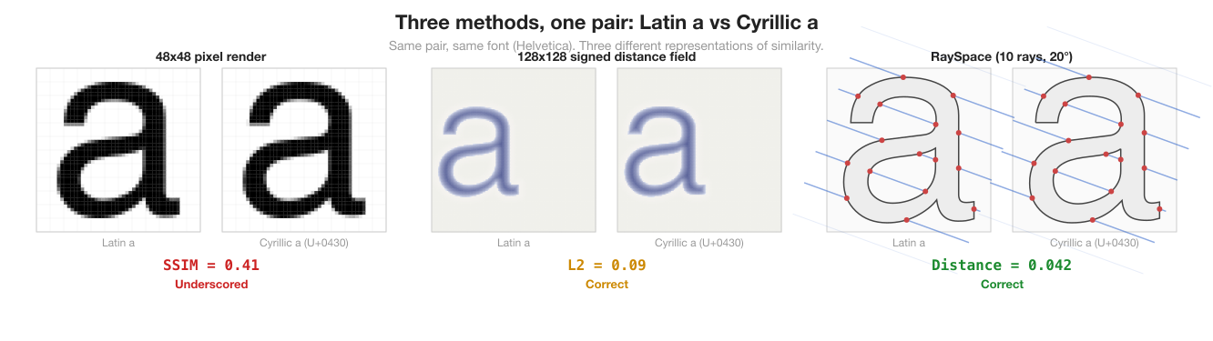
More fundamentally, SSIM underscored the pairs that matter most. Cyrillic а (U+0430) vs Latin a (U+0061), the canonical cross-script confusable, scored SSIM 0.41. These characters share identical outlines in most sans-serif fonts. SSIM scored them at 0.41 because minor rendering differences (anti-aliasing, pixel grid alignment) created structural noise that the algorithm interpreted as dissimilarity. The signed distance field (SDF) approach that replaced SSIM scored the same pair at NCC 0.95, much closer to the geometric reality.
SSIM also struggled with small features. The dot on “i”, accent marks, and diacritics shifted SSIM scores by amounts that swamped the structural signal. A character with a dot above it and the same character without the dot might score 0.85, high enough to flag as confusable. The dot is 4 pixels in a 48x48 grid. It should not dominate the comparison.
The SDF detour
The replacement was signed distance fields. For each character, compute a 128x128 grid where each cell stores the signed distance from that point to the nearest outline edge. Negative values are inside the glyph, positive outside. Compare two grids with L2 (root-mean-square difference) and NCC (normalised cross-correlation).
SDF solved the accuracy problem. Cyrillic а vs Latin a: L2 = 0.000, NCC = 1.0 in Tahoma. The outlines are identical; the metric reflects that. The cross-script discovery pipeline used SDF to find 41,680 unique confusable pairs across 245 fonts.
But SDF introduced a new bottleneck. Computing a 128x128 distance field means evaluating the distance from 16,384 grid points to every Bezier segment in the outline. A typical Latin character has 20-40 segments. A Han character can have 200+. Each distance evaluation involves finding the closest point on a quadratic or cubic Bezier curve. Not cheap. SDF was the right metric but too slow to use as a first-pass filter.
The pipeline used raycasting as a pre-filter: cast rays through outlines, count intersections, reject pairs with different topology. Then run SDF only on the survivors. This three-stage cascade (width filter, raycasting filter, SDF scoring) reduced 52 million comparisons to 449,000 SDF evaluations. The raycasting filter was doing 72% of the work.
The question became: if raycasting is already capturing structural similarity well enough to filter, can it replace SDF entirely?
The idea has a lineage
The application is new, but the underlying principles are not. Raycasting draws from a deep well of prior work across domains that all share one principle: you can characterize geometry by firing directed energy along straight lines and analysing what comes back.
John Carmack (1992) made raycasting fast. Wolfenstein 3D cast one ray per screen column through a 2D grid map. The distance to the first wall hit determined the wall height. A year later, Doom replaced the grid with arbitrary 2D geometry and added height variation, but the core insight was the same: parallel rays through a 2D structure, intersection distances encoding shape. RaySpace applies that trade: glyph outlines are 2D, rays are 1D, and the intersection pattern encodes enough structural information to compare shapes without ever reconstructing an image.
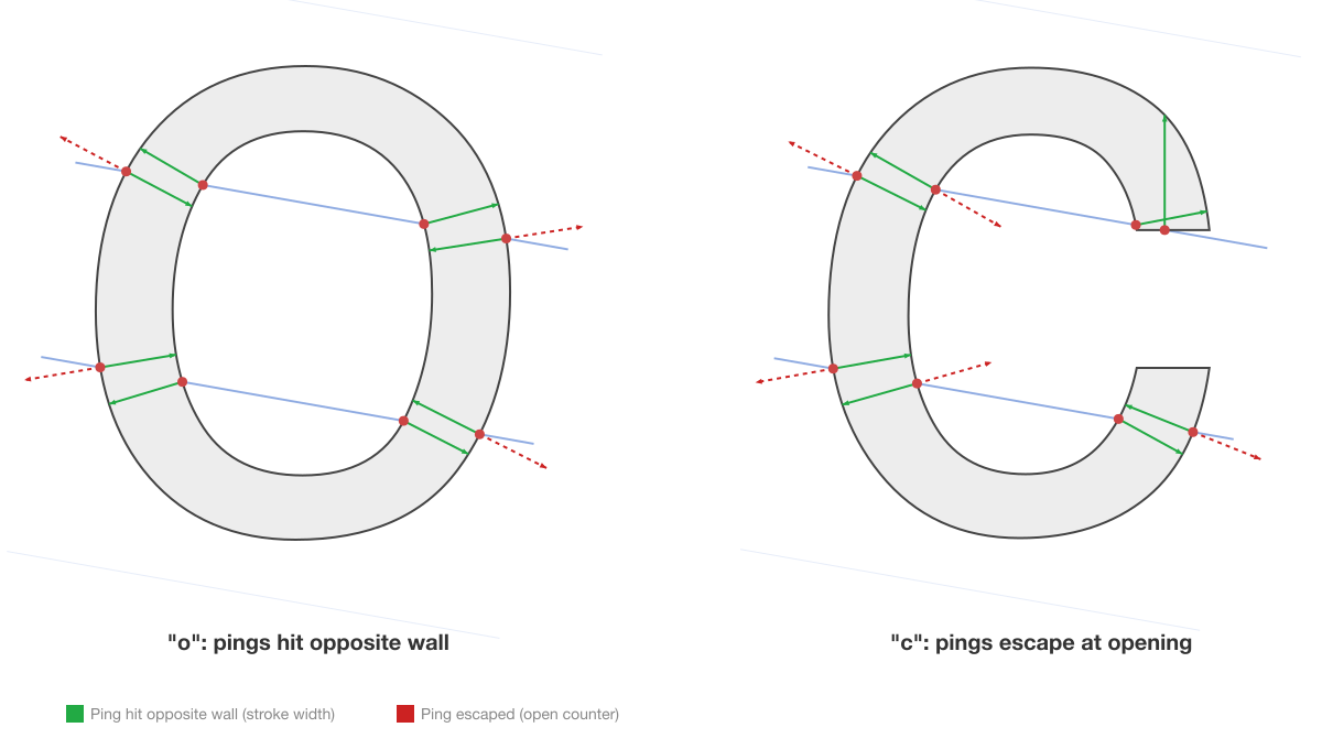
Ambient occlusion (1998/2002) is the ancestor of ping rays. AO asks “how enclosed is this surface point?” by casting rays outward and measuring what fraction hit nearby geometry. Ping rays ask the same question in 2D: fire perpendicular to the outline, measure the distance to the opposite wall. Short = thin stroke. Long = wide counter. Escape = opening (the difference between “c” and “o”).
Computed tomography provides the mathematical guarantee. Radon proved in 1917 that the complete set of line integrals through a 2D function uniquely determines that function. RaySpace is a discretised binary Radon transform. Even a coarse approximation (36 angles, 50 rays) captures enough information to distinguish most shapes. This is why multi-angle ray probing works: Radon’s theorem guarantees it.
None of this was planned. The raycasting filter existed before I recognised the connections. The technique is new in its application (nobody has raycasted font outlines for confusable detection before), but the principles are 50 to 100 years old. The full lineage, from Appel’s 1968 ray probe through acoustic impulse responses to CT sinograms, is covered in the companion post on prior art.
Raycasting: the core idea
Cast a line through a glyph outline. Count how many times it crosses the boundary. A vertical stroke produces 2 crossings (entry, exit). The letter “o” produces 4 crossings (outer entry, inner entry, inner exit, outer exit). The letter “c” produces 2 crossings at most angles but 0 at the angle that passes through the gap.
Do this at 36 angles (0 to 175 degrees, 5-degree steps) with 50 parallel rays per angle. Each glyph produces 1,800 intersection counts: a topological fingerprint that captures how many strokes, counters, and holes exist at every projection angle.
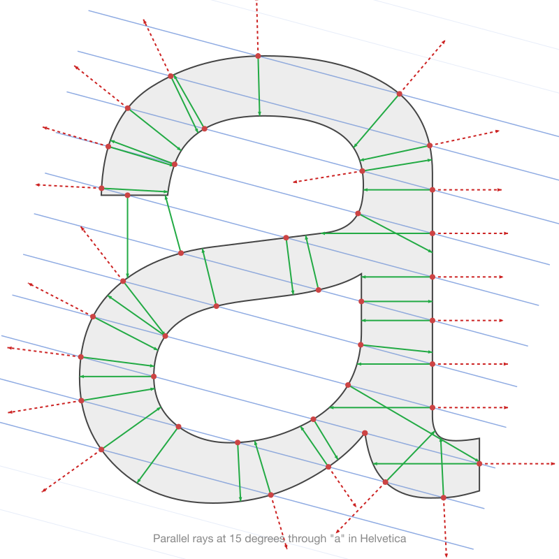
The short green and red arrows at each intersection are ping rays, perpendicular probes that measure stroke width. They are explained in the next section.
Two characters with the same topological structure produce similar count patterns. Latin o and Cyrillic o: identical counts at every angle. Latin “l” and Arabic alef in Tahoma: identical counts at every angle (both are single vertical strokes in that font). The count signature captures this immediately, with no rendering.
But counts alone have blind spots.
The five layers
Intersection counts were the first implementation. They worked for gross structural comparison but failed on two classes of pairs:
The dot problem. Latin “i” vs Arabic alef. The dot on “i” adds 2 extra crossings (entry + exit) at rays that pass through it, roughly 13% of all rays. Averaging across 1,800 rays dilutes this signal below any useful threshold. The count-only metric scored i/alef at 0.37, indistinguishable from genuinely similar pairs.
The open-vs-closed problem. Latin “c” vs “o”. At most angles, both produce 2 crossings (entry, exit) or 4 crossings (with counter). The difference is that “c” has an opening where rays pass through without crossing. But this only affects a narrow range of angles. Count-only scored c/o at 0.34.
The solution was not to discard counts but to add more layers of information from the same rays. Each ray already computes exact intersection points against every Bezier segment. The count-only pipeline was throwing away everything except the count. RaySpace keeps five layers:
| Layer | Signal | What it captures |
|---|---|---|
| Counts | How many crossings | Topology: strokes, holes, counters |
| Positions | Where crossings occur | Spatial layout of strokes |
| Crossing angles | Ray vs. tangent angle | Stroke direction at each hit |
| Ping distances | Perpendicular probe inward | Stroke width |
| Ping depth | Longer perpendicular probe | Counter depth, open vs. closed |
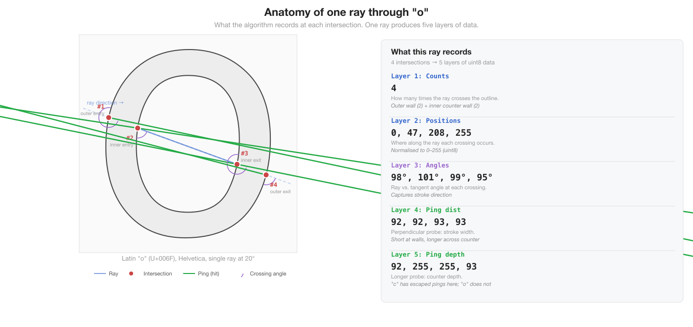
Layer 1: Counts. How many times the ray crosses the outline. The original topological fingerprint. Stored as uint8 (0-255), capped at 10 per ray.
Layer 2: Positions. Where along the ray each crossing occurs, normalised to [0, 1] relative to the glyph bounding box and quantised to uint8. Two characters with the same count but different intersection positions (like c vs o at angles where both have 2 crossings) now produce different signatures.
Layer 3: Crossing angles. The angle between each ray and the outline tangent at the intersection point. A ray crossing a vertical stroke at 90 degrees produces a different signal than one crossing a diagonal stroke at 45 degrees. This captures stroke direction: whether the outline is curving left, right, or running straight at each intersection.
Layer 4: Ping distances. At each intersection, a secondary “ping” ray fires perpendicular to the outline tangent, into the glyph interior. The distance it travels before hitting the opposite wall measures local stroke width. A thin stroke (like the vertical of “l”) produces a short ping distance. A wide bowl (like the counter of “o”) produces a long one. Stored as uint8, 255 = ping escaped without hitting anything.
Layer 5: Ping depth. The same perpendicular ping ray, but measuring the longer of the two directions (both normals are tested). This captures counter depth: how much open space exists on the other side of the stroke. In the letter “o”, pings from the outer wall hit the inner wall (short, measuring stroke width) but pings from the inner wall in the opposite direction measure the counter depth (longer). The ratio of ping distance to ping depth distinguishes thick strokes from thin ones and solid regions from open counters.
The ping rays are what separate RaySpace from simple raycasting. Counts and positions capture topology (how many strokes, where they are). Crossing angles capture orientation (which direction strokes run). Pings capture geometry (how thick strokes are, how deep counters are). Together, these five layers describe the interior structure of a glyph at sub-stroke resolution.
Each glyph produces five uint8 arrays. Counts and positions are variable-length (positions has sum(counts) elements). Crossing angles, ping distances, and ping depth each have one element per intersection. The total signature for a typical Latin character is approximately 5,400 values.
Comparison metric
Two RaySpace signatures are compared ray by ray. For each of the 1,800 rays, one of three cases applies:
| Case | Condition | Distance |
|---|---|---|
| Both miss | countA == 0 and countB == 0 | 0 |
| Same count | countA == countB > 0 | MSE of sorted position/angle/ping values |
| Different count | countA != countB | MSE of matched positions + 1.0 per unmatched |
The 1.0 unmatched penalty is a deliberate design choice. An unmatched intersection means one glyph has a structural component (stroke, dot, accent) that the other lacks. This should dominate the distance. Without this penalty, the dot on “i” contributes a small fractional difference averaged across 1,800 rays. With it, each of the ~234 rays that pass through the dot contributes a full 1.0, a signal that cannot be diluted by averaging.
Per-ray distances within each angle are averaged to produce 36 per-angle scores. These are combined with a mean-max blend:
Mean alone fails for localised features (the dot affects 12 of 36 angles; pure mean divides the signal by 3). Max alone is too sensitive to noise. The blend preserves peak signals while keeping the overall score stable.
What it finds
True confusables: Latin o vs Cyrillic o
The ground truth test. Latin o (U+006F) and Cyrillic o (U+043E) share identical outlines in most fonts. RaySpace scores them at 0.000 in Tahoma and Arial. In Helvetica, where the outlines have sub-curve differences, the score is 0.020, still well within the confusable range.
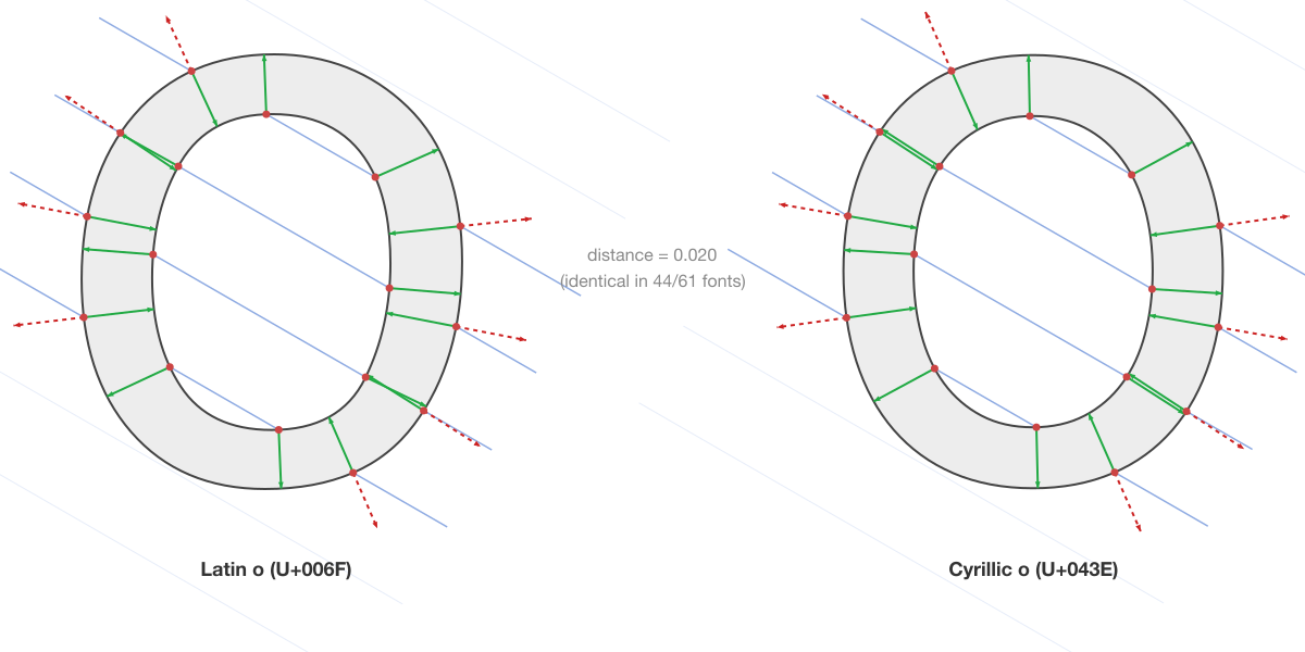
This is what a true confusable looks like in RaySpace: identical intersection patterns at every angle, identical positions, identical ping distances. The metric reflects the geometric reality that these are the same curves.
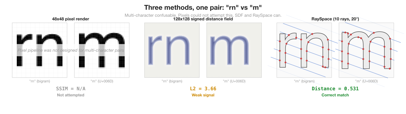
Multi-character: “rn” vs “m”
The textbook multi-character confusable. The pipeline concatenates the outlines of “r” and “n” (with font kerning applied) and compares against “m” as a single glyph. RaySpace scores this at 0.253 in InaiMathi, 0.296 in Heiti SC, 0.333 in Arial.
This is also where the three methods diverge most clearly. The pixel pipeline (SSIM) was never designed for multi-character comparison: it had no mechanism to concatenate two characters and score them against one. SDF can handle it, but the L2 distance (3.66 in Helvetica) is 40x higher than single-character confusables (0.09 for a/а), meaning you need separate thresholds for single-char and multi-char comparisons. RaySpace’s distance (0.531) is on the same continuous scale as all other comparisons. The same threshold logic works for both.
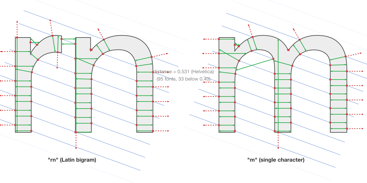
The per-font variation is the point. In sans-serif fonts with uniform stroke weight (Arial, Helvetica, System Font), “rn” and “m” are nearly identical: the arches of n align with the arches of m, and the junction between r and n is barely visible. In serif fonts (Didot at 0.910, Baskerville at 0.881) or decorative fonts (Savoye LET at 1.394), the difference is obvious. A detection system that knows the user’s font can set an appropriate threshold instead of treating all fonts the same.
The top 10 fonts for rn/m confusion:
| Font | RaySpace distance |
|---|---|
| InaiMathi | 0.253 |
| Heiti SC | 0.296 |
| Shree Devanagari 714 | 0.297 |
| Khmer Sangam MN | 0.298 |
| Arial Narrow | 0.316 |
| System Font | 0.316 |
| Arial Unicode MS | 0.317 |
| Heiti TC | 0.321 |
| Microsoft Sans Serif | 0.332 |
| Arial | 0.333 |
33 fonts score below 0.40. 65 below 0.60. 95 fonts total produce a match. These are the fonts where rn/m substitution is hardest to detect visually.
Novel discoveries
Multi-character. The bigram pipeline searched 190 million combinations (676 Latin bigrams x 294,646 bank targets x 245 fonts). At RaySpace distance < 2.0 (a deliberately wide net for discovery, not a confusability claim), it surfaced 2,866,184 unique candidate pairs. No previous system attempted this search.
The multichar post documents the 571,753 candidates from the earlier SDF pipeline (L2 < 15.0, similarly generous); the enriched five-layer signature recovered the remainder by correcting false rejections in the count-only pre-filter.
Consumers filter to their desired confidence: distance < 0.5 for high-confidence confusables, < 1.0 for probable matches. The results include cross-script bigram matches where a Latin two-character sequence resembles a single character from another script:
Latin bigrams matching Cyrillic characters: “bl” matches Cyrillic ы (yeru) across 49 fonts. “rl” matches Cyrillic л (el) across 22 fonts. “ro” matches Cyrillic ю (yu) across 26 fonts.
Latin “ll” matches Devanagari double danda (U+0965) at 0.176 across 8 fonts. Two vertical strokes match two vertical strokes.
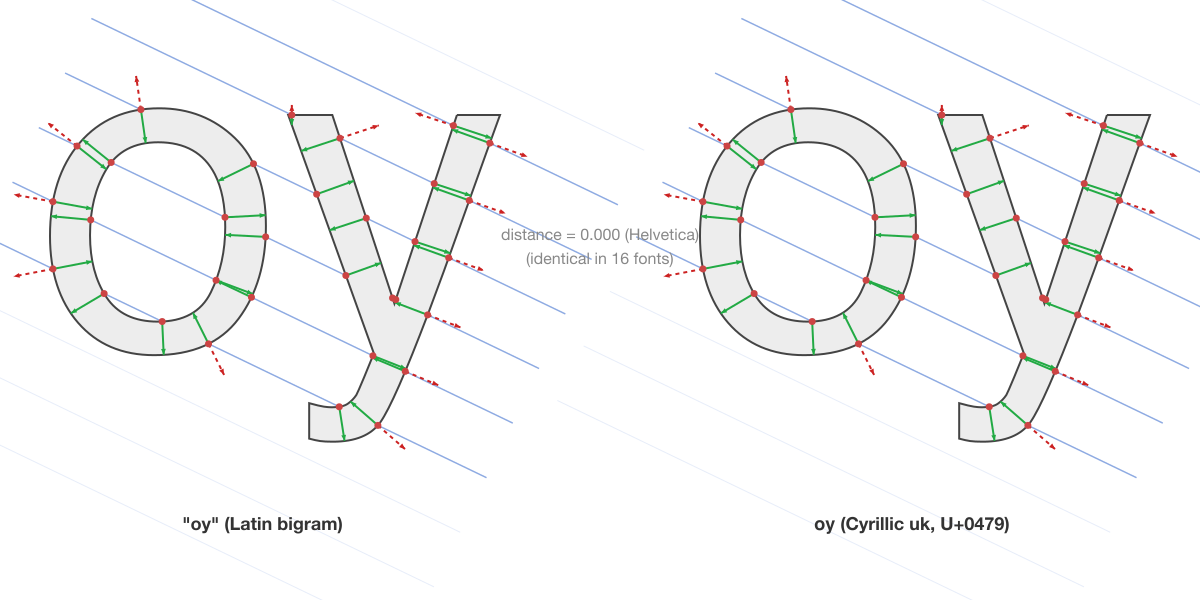
Latin “oy” matches Cyrillic ѹ (uk, U+0479) at distance 0.000 in Helvetica, confirmed across 16 fonts. Geometrically perfect but practically harmless: U+0479 has IdentifierType=Obsolete and cannot appear in identifiers or domain names. It illustrates the kind of exotic match the pipeline surfaces, and why IDN relevance filtering matters.
Single-character recovery. The enriched five-layer signature recovered 19,983 cross-script pairs that the earlier count-only raycasting filter had been incorrectly rejecting. These all passed SDF scoring when tested directly. The count-only filter was too aggressive; the additional layers (positions, crossing angles, pings) preserved the structural signal needed to identify them.
East Asian coverage gaps. The single-character discoveries revealed a systematic blind spot in Unicode’s confusables.txt. Latin/Cyrillic is well-covered: the canonical pairs (o/о, a/а, c/с) are all listed. East Asian cross-script pairs are not. confusables.txt includes four Han-Katakana pairs (口/ロ, 二/ニ, 卜/ト, 工/エ), but RaySpace found 752 Recommended Han-Katakana pairs at mean distance < 1.0, with 15 at high confidence (mean < 0.5). Japanese is the one major script context where mixed-script domain labels are legitimate: Japanese labels routinely combine Han, Katakana, Hiragana, and Latin. The pairs that existing systems miss are exactly the pairs that could appear together in a valid label. The IDN relevance analysis traces the full filtering from 250K pairs to 102 at high confidence.
Why not SDF?
SDF was good. RaySpace is better on three axes:
Speed. RaySpace computes a glyph signature in a single pass over the outline segments. SDF requires evaluating 16,384 grid points against every segment. For a character with 40 segments, SDF performs 655,360 closest-point-on-Bezier evaluations. RaySpace performs 1,800 ray-segment intersection tests (36 angles x 50 rays), each of which is a simple quadratic or cubic solve. For the multichar discovery pipeline (190 million comparisons), RaySpace completes in 63 minutes. SDF needed 91 minutes for the same search space, with raycasting doing the heavy filtering anyway.
Information density. SDF produces a 128x128 grid (16,384 values per glyph). RaySpace produces ~5,400 values per glyph with more structural resolution. SDF captures the distance field uniformly, spending equal resolution on empty space and dense stroke regions. RaySpace concentrates information at the outline boundary where the structural signal lives.
Ping rays have no SDF equivalent. SDF measures distance to the nearest edge at grid points. It does not capture the relationship between opposing edges of a stroke: the stroke width, counter depth, or whether a ping ray escapes through an opening. These are the signals that distinguish “c” from “o” and thick strokes from thin ones.
The comparison between pipelines is definitive, measured at the same discovery threshold (distance < 2.0, a wide net). On the cross-script task, RaySpace surfaced 61,663 unique candidate pairs where the SDF pipeline found 41,680 (a 48% increase). On multi-character discovery, RaySpace surfaced 2,866,184 candidates where the SDF pipeline (count-only pre-filter + L2 < 15.0) found 571,753 (a 401% increase). The additional pairs all passed SDF scoring when tested directly. The count-only raycasting pre-filter had been incorrectly rejecting them; the enriched five-layer signature corrected that.
The filter cascade
RaySpace does not eliminate the need for filtering. The full pipeline uses a two-stage cascade:
The width filter is the cheapest check: if two characters have advance widths that differ by more than 15%, they cannot be confusable regardless of shape. This eliminates 27% of pairs with a single comparison. The RaySpace filter handles the remaining 73%, reducing to 1.6% of the original search space. No SDF step.
For multi-character discovery (676 Latin bigrams x 294,646 bank targets x 245 fonts = 190 million comparisons), the cascade is even more effective:
The width filter alone eliminates 63.3%. Most single characters have advance widths nothing like a two-character sequence. The bigrams that survive are compared using the full five-layer RaySpace signature.
The signature bank
Comparing 22,581 characters across 245 fonts means computing 294,646 RaySpace signatures (one per font/codepoint pair with glyph coverage). Rather than recompute these for every query, the pipeline pre-builds a signature bank.
The bank is a 2.55 GB gzip-compressed JSONL file. Each line contains one entry: codepoint, font name, advance width, and the five uint8 arrays (counts, positions, crossing angles, ping distances, ping depth). Loading the bank takes approximately 300 seconds and consumes ~2.1 GB of heap memory, using Uint8Array typed arrays instead of standard JavaScript number[] to fit within the 8 GB heap limit.
The bank enables O(1) lookup for any glyph comparison. The discovery pipeline loads the bank once, then compares each query signature against all relevant targets using array arithmetic. No font loading, no outline extraction, no signature computation at query time.
What this means
RaySpace makes three things possible that were not before:
Per-font confusable scoring. The distance between any two characters depends on the font. “rn” and “m” in Arial: 0.333. In Didot: 0.910. A detection system that knows the user’s font can adapt its sensitivity. This is the core capability that font-specific confusable maps are built on.
Multi-character detection at scale. Checking whether a two-character sequence matches a single character requires comparing concatenated outlines against every candidate target in the user’s font. RaySpace makes this fast enough to search 190 million combinations in an hour. The multichar post documents the initial 571,753 SDF-scored candidates; the enriched five-layer signature expanded that to 2.87 million candidates at the same discovery threshold, with consumers filtering to their desired confidence level.
Systematic coverage gaps. The 249,976 single-character discoveries revealed where existing confusable databases are thin. Latin/Cyrillic is well-covered in confusables.txt. East Asian cross-script pairs are not: RaySpace found 752 Recommended Han-Katakana pairs at mean distance < 1.0, most absent from confusables.txt. Japanese is the one context where mixed-script domain labels are legitimate, making these the most security-relevant omissions. The IDN relevance analysis traces the filtering.
The scored datasets feed namespace-guard for runtime confusable detection. The methodology is open source in confusable-vision.
For a detailed survey of prior work in confusable detection and shape analysis, and where RaySpace fits in that landscape, see the companion post on prior art.
How to reproduce
git clone https://github.com/paultendo/confusable-vision
cd confusable-vision
npm install

# Build signature bank (~45 min, one-time)
npx tsx scripts/build-signature-bank.ts

# Single-character cross-script discovery (~86 min)
npx tsx scripts/discover-singlechar-sdf.ts --scorer=ray

# Multi-character bigram discovery (~63 min)
npx tsx scripts/discover-multichar-sdf.ts --scorer=ray

# Output: data/output/*.jsonl
Requires macOS with system fonts (245 fonts on a standard install). The pipeline is portable to other platforms with different font sets.